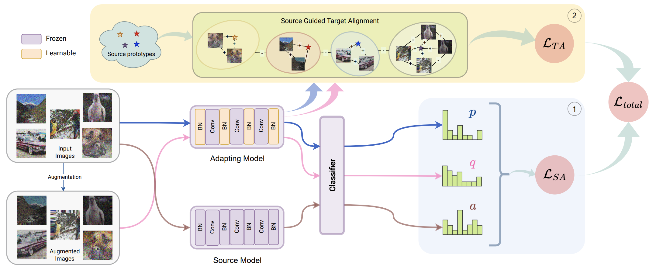
Only the BN affine parameters of the adapting model \( f_\theta \) are updated during test time. The adapting model is initialised from the source model \( f_{\theta_s} \). At each step, both models have their BN statistics updated to match the current test batch statistics; the source-corrected model is called the Target Corrected Source (TCS) model \( f_{\theta_s}^k \). SANTA has two components:
The TCS model provides domain-invariant predictions for the current batch. We use its outputs as soft anchors for the adapting model via self-distillation. Let \( p_{ij} \) and \( a_{ij} \) denote the \( j \)-th class scores from the adapting and TCS models for image \( x_i \). The base source-anchoring loss is:
\[ \mathcal{L}'_{SA} = -\frac{1}{N}\sum_{i=1}^{N}\sum_{j=1}^{C} p_{ij} \log(a_{ij}) \tag{1} \]
Using augmented copies of the test images makes the model more robust. Let \( q_{ij} \) be the adapting model's score for the augmented version. The complete SA loss is:
\[ \mathcal{L}_{SA} = -\frac{1}{N}\sum_{i=1}^{N}\sum_{j=1}^{C} \left( p_{ij}\log(a_{ij}) + q_{ij}\log(a_{ij}) \right) \tag{2} \]
This avoids storing a separate teacher model, requires no restoration hyperparameter, and directly uses the adapting model for prediction.
The goal is to make features gradually domain-invariant as the model encounters data from different domains. The adapting model \( f_\theta^k = h \circ g_\phi^k \) is decomposed into a feature extractor \( g_\phi^k \) and a fixed classifier \( h \). Features are projected to a \( d \)-dimensional hypersphere:
\[ z_i = p_\psi \circ g_\phi^k(x_i) \tag{3} \]
The base contrastive loss pairs each sample with its augmented view:
\[ \mathcal{L}_{con} = \frac{1}{N}\sum_{i=1}^{N} \log \frac{\exp(z_i \cdot z_{N+i}/\tau)}{\sum_{k=1, k\neq i}^{2N}\exp(z_i \cdot z_k/\tau)} \tag{4} \]
To ensure target clusters align with the source feature space, the nearest source prototype \( \pi(x_i) \) is used as a third view:
\[ \pi(x_i) = \{\pi_t \mid t = \arg\max_c \cos(\pi_c,\, g_\phi^k(x_i))\} \tag{5} \]
The source prototype guided Target Alignment loss uses two positive views per sample (augmented image + nearest source prototype):
\[ \mathcal{L}_{TA} = \frac{1}{2N}\sum_{i=1}^{N}\left[\log \frac{\exp(z_i \cdot z_{N+i}/\tau)}{\sum_{k\neq i}^{3N}\exp(z_i \cdot z_k/\tau)} + \log \frac{\exp(z_i \cdot z_{2N+i}/\tau)}{\sum_{k\neq i}^{3N}\exp(z_i \cdot z_k/\tau)}\right] \tag{6} \]
The BN affine parameters \( \phi \) and projection head \( \psi \) are updated at each test batch by minimizing:
\[ \mathcal{L}_{SANTA} = \mathcal{L}_{SA} + \mathcal{L}_{TA} \tag{7} \]
The adapting model is used directly for prediction and is robust enough to update continuously without any restoration back to the source model.