ROSITA

Abstract

Adapting models to dynamic, real-world environments characterized by shifting data distributions and unseen test scenarios is a critical challenge in deep learning. In this paper, we consider a realistic and challenging Test-Time Adaptation setting, where a model must continuously adapt to test samples that arrive sequentially, one at a time, while distinguishing between known and unknown classes. Current Test-Time Adaptation methods operate under closed-set assumptions or batch processing, differing from the real-world open-set scenarios. We address this limitation by establishing a comprehensive benchmark for Open-set Single-image Test-Time Adaptation using Vision-Language Models. Furthermore, we propose ROSITA, a novel framework that leverages dynamically updated feature banks to identify reliable test samples and employs a contrastive learning objective to improve the separation between known and unknown classes. Our approach effectively adapts models to domain shifts for known classes while rejecting unfamiliar samples. Extensive experiments across diverse real-world benchmarks demonstrate that ROSITA sets a new state-of-the-art in open-set TTA, achieving both strong performance and computational efficiency for real-time deployment.

Problem Setting

We consider Open-set Single-image Test-Time Adaptation (OSTTA): at each time step \(t\), a single test sample \(x_t\) arrives from a stream \(\mathcal{D}_t = \mathcal{D}_d \cup \mathcal{D}_u\) comprising:

Desired class samples \(\mathcal{D}_d\): from one of the \(|\mathcal{C}_d|\) known classes, potentially under domain shift.
Undesired class samples \(\mathcal{D}_u\): from unknown classes \(\mathcal{C}_u\), with \(\mathcal{C}_d \cap \mathcal{C}_u = \emptyset\) (semantic shift).

The goal is to perform \(|\mathcal{C}_d| + 1\) way classification at each step: identify whether \(x_t\) is a desired class sample, and if so, classify it correctly; otherwise predict "I don't know." Unlike prior TTA work, there is no batch, no source data, and no ground-truth labels — the model must adapt on a single image at a time under a continuously shifting mix of domain and semantic shift.

We evaluate under four OSTTA scenarios:

Single domain: desired samples from one unseen domain + undesired samples.
Continuously changing domains: desired domain shifts over time.
Frequently changing domains: very few samples per domain.
Varying sample ratio: different proportions of desired vs. undesired samples.

Proposed Method: ROSITA

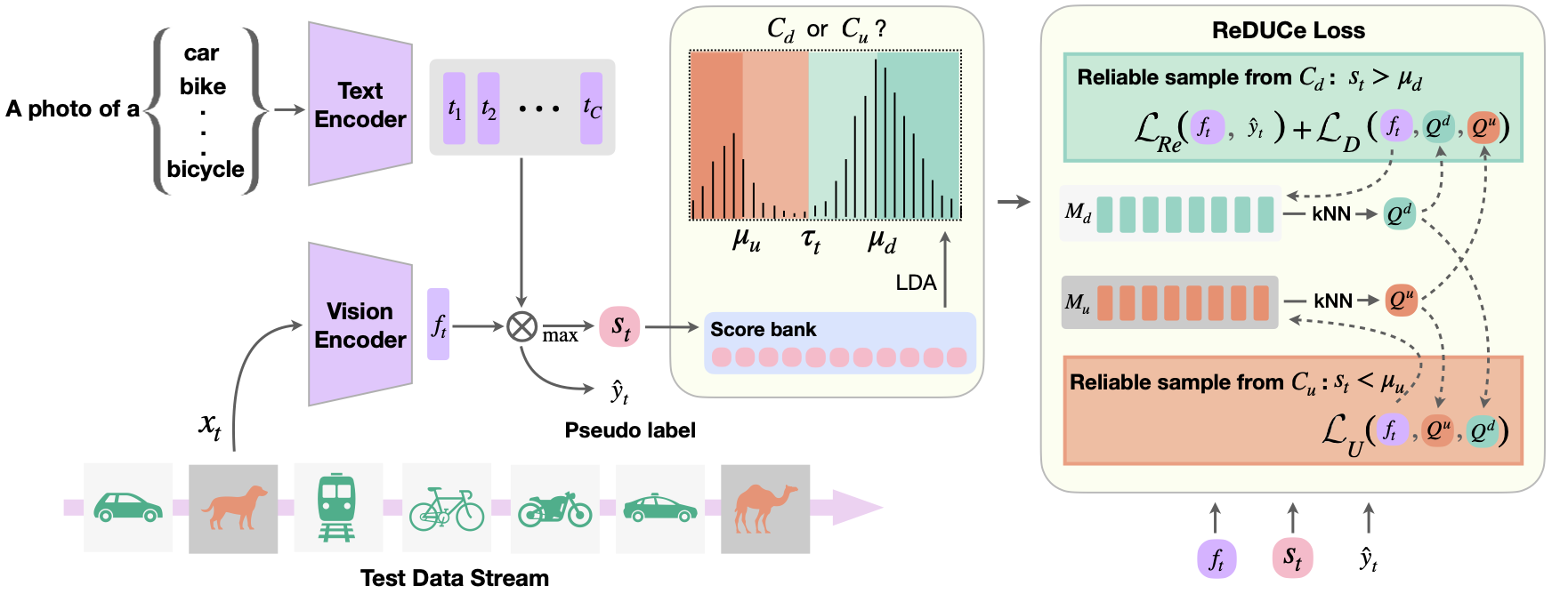
ROSITA uses CLIP as its backbone and adapts only the LayerNorm parameters of the Vision Encoder — a lightweight and stable choice confirmed by systematic analysis across 7 parameter groups. The framework has two components: an LDA-based desired/undesired class identifier and the ReDUCe contrastive loss.

ROSITA framework overview — **ROSITA framework:** Test samples from \(\mathcal{C}_d\) and \(\mathcal{C}_u\) arrive one at a time. An LDA-based identifier classifies each sample as desired or undesired. If reliable, the respective feature bank is updated and the ReDUCe loss optimizes the LayerNorm parameters of the Vision Encoder.

Desired vs. Undesired Class Identifier

Each sample's maximum cosine similarity score with the text classifiers is computed:

\[ s_t = \max_k\; \text{sim}(f_t,\, t_k) \tag{1} \]

A dynamic threshold \(\tau^*_t\) is found via LDA over a continuously updated score bank \(\mathcal{S}\), minimizing within-group variance:

\[ \tau^*_t = \arg\min_\tau \left[\frac{1}{|\mathcal{S}_d|}\sum_{s\in\mathcal{S}_d}(s-\mu_d)^2 + \frac{1}{|\mathcal{S}_u|}\sum_{s\in\mathcal{S}_u}(s-\mu_u)^2\right] \tag{2} \]

A sample is classified as desired if \(s_t \geq \tau^*_t\), undesired otherwise. Samples near the threshold are treated as unreliable and do not trigger adaptation.

ReDUCe Loss

Two feature banks \(\mathcal{M}_d\) (desired, size \(|\mathcal{C}_d| \times K\)) and \(\mathcal{M}_u\) (undesired, size 64) are updated dynamically. For each reliable sample, \(K\)-nearest neighbours are retrieved: \(Q_d = \text{kNN}(f_t;\, \mathcal{M}_d)\), \(Q_u = \text{kNN}(f_t;\, \mathcal{M}_u)\).

For a reliable desired sample (\(s_t > \mu_d\)), two losses are applied:

\[ \mathcal{L}_{Re} = \mathcal{L}_{CE}(x_t,\hat{y}_t) + \mathcal{L}_{CE}(\tilde{x}_t,\hat{y}_t) \tag{3} \]

\[ \mathcal{L}_D = -\frac{1}{K^+}\sum_{z^+\in Q_d}\mathbf{1}(y^+=\hat{y}_t)\log\frac{\exp(\text{sim}(f_t,z^+)/\tau)}{\sum_{z^-\in Q_u}\exp(\text{sim}(f_t,z^-)/\tau)} \tag{4} \]

For a reliable undesired sample (\(s_t < \mu_u\)):

\[ \mathcal{L}_U = -\frac{1}{K}\sum_{z^+\in Q_u}\log\frac{\exp(\text{sim}(f_t,z^+)/\tau)}{\sum_{z^-\in Q_d}\exp(\text{sim}(f_t,z^-)/\tau)} \tag{5} \]

The full ReDUCe objective is:

\[ \mathcal{L}_{ReDUCe} = \begin{cases} \mathcal{L}_{Re} + \mathcal{L}_D & \text{if } s_t > \mu_d \\ \mathcal{L}_U & \text{if } s_t < \mu_u \end{cases} \tag{6} \]

The gradient of \(\mathcal{L}_D\) attracts \(f_t\) toward positive desired-class neighbours while repelling it from undesired neighbours (with hard negatives exerting stronger repulsion), progressively sharpening the decision boundary.

Results

Open-set TTA on ImageNet-scale Benchmarks

Method	IN-C / MNIST		IN-C / SVHN		IN-R / MNIST		IN-R / SVHN
Method	AUC↑	AccHM↑	AUC↑	AccHM↑	AUC↑	AccHM↑	AUC↑	AccHM↑
ZS-Eval	93.39	41.43	85.89	40.83	91.27	71.50	90.43	71.66
TPT	93.12	42.21	85.43	40.95	91.25	71.98	90.43	72.36
(K+1)PC	95.76	42.95	87.75	38.50	97.46	81.51	97.55	80.39
UniEnt	94.19	41.53	87.56	41.10	91.64	71.73	90.86	71.96
TDA	90.54	43.66	86.76	43.07	91.79	71.56	90.67	71.48
ROSITA	99.52	48.53	98.34	46.32	99.44	83.53	98.62	80.75

Table 1: Open-set TTA results (CLIP ViT-B/16) with ImageNet-C and ImageNet-R as desired domains, MNIST and SVHN as undesired. ROSITA achieves the best AUC across all settings, with large gains in FPR (not shown) indicating far fewer false positives.

AccHM on VisDA and DomainNet-126

Method	VisDA	Clipart	Painting	Sketch
ZS-Eval	78.28	50.22	47.81	48.59
TPT	78.42	57.71	49.73	54.67
(K+1)PC	90.35	71.21	70.61	67.21
UniEnt	78.09	57.88	49.75	54.76
TDA	76.85	61.04	51.20	55.26
ROSITA	90.64	71.40	70.89	67.35

Table 2: AccHM (%) with VisDA and DomainNet-126 domains as desired data (\(\mathcal{D}_d\)) and MNIST as undesired (\(\mathcal{D}_u\)). ROSITA matches or surpasses all methods by a large margin.

Ablation: ReDUCe Loss Components

\(\mathcal{L}_{Re}\)	\(\mathcal{L}_D\)	\(\mathcal{L}_U\)	CIFAR-10C / MNIST		ImageNet-R / MNIST
			AUC↑	AccHM↑	AUC↑	AccHM↑
			91.91	75.57	91.27	71.50
✓			95.29	80.97	81.07	64.32
		✓	98.61	79.84	99.39	80.82
	✓	✓	99.27	80.69	99.48	81.92
✓	✓	✓	99.10	84.17	99.44	83.53

Table 3: Ablation of ReDUCe loss components (CLIP ViT-B/16). Each term contributes: \(\mathcal{L}_U\) provides the largest AUC boost on IN-R/MNIST; the full combination yields the best AccHM on both settings.

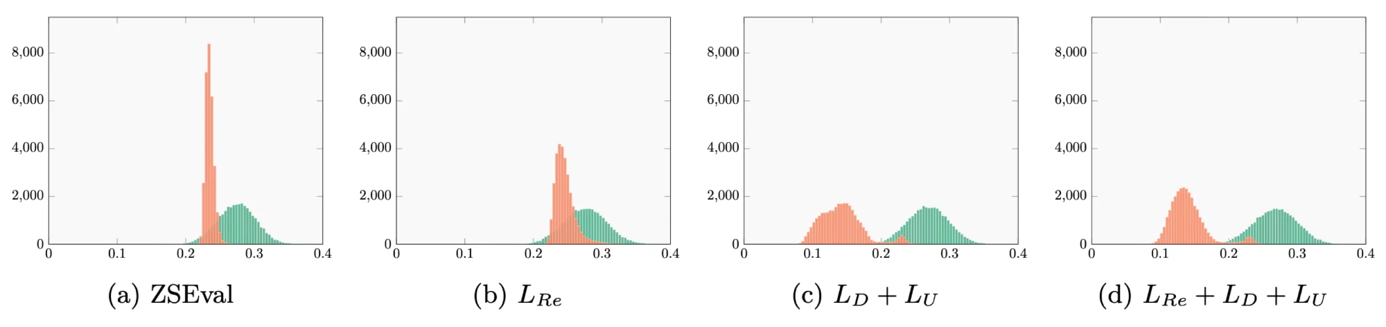
Score histograms showing effect of ReDUCe loss components — Histograms of desired (\(\mathcal{C}_d\), orange) and undesired (\(\mathcal{C}_u\), green) class scores on CIFAR-10C / MNIST for different loss configurations. (a) ZSEval: classes heavily overlap. (b) \(\mathcal{L}_{Re}\) alone: slight separation. (c) \(\mathcal{L}_D + \mathcal{L}_U\): bimodal split emerges. (d) Full ReDUCe (\(\mathcal{L}_{Re} + \mathcal{L}_D + \mathcal{L}_U\)): clear separation achieved.

BibTeX

@article{sreenivas2025rosita,
  author  = {Sreenivas, Manogna and Biswas, Soma},
  title   = {Efficient Open Set Single Image Test Time Adaptation of Vision Language Models},
  journal = {Transactions on Machine Learning Research},
  year    = {2025}
}

Effectiveness of Vision Language Models for Open-world Single Image Test Time Adaptation