PhISH-Net

Abstract

Underwater imaging presents numerous challenges due to refraction, light absorption, and scattering, resulting in color degradation, low contrast, and blurriness. Enhancing underwater images is crucial for high-level computer vision tasks, but existing methods either neglect the physics-based image formation process or require expensive computations. In this paper, we propose an effective framework that combines a physics-based Underwater Image Formation Model (UIFM) with a deep image enhancement approach based on the retinex model. Firstly, we remove backscatter by estimating attenuation coefficients using depth information. Then, we employ a retinex model-based deep image enhancement module to enhance the images. To ensure adherence to the UIFM, we introduce a novel Wideband Attenuation prior. The proposed PhISH-Net framework achieves real-time processing of high-resolution underwater images using a lightweight neural network and a bilateral-grid-based upsampler. Extensive experiments on two underwater image datasets demonstrate the superior performance of our method compared to state-of-the-art techniques.

Problem Setting

Underwater images are degraded by two physical effects: (i) direct signal attenuation, where colors are absorbed differently by water as a function of depth and wavelength (red absorbed more than blue/green); and (ii) backscatter, from light scattered by suspended particles toward the camera. We follow the UIFM from Sea-Thru, which models any captured image \(I\) per channel \(c \in \{r,g,b\}\) as:

\[ I_c = D_c + B_c \tag{1} \]

\[ I = J \cdot e^{-\beta_d z} + B^\infty (1 - e^{-\beta_b z}) \tag{2} \]

Here \(J\) is the unattenuated scene, \(z\) is depth, \(\beta_d\) is the wideband attenuation coefficient, \(\beta_b\) is the backscatter coefficient, and \(B^\infty\) is the background backscatter color. The goal is to recover \(J\) from \(I\) and a depth map \(z\).

Sample PhISH-Net enhancement results from UIEB dataset — **Fig. 1:** Sample results on the UIEB dataset. **Top:** input underwater images; **Bottom:** corresponding PhISH-Net enhanced outputs.

Proposed Method: PhISH-Net

Backscatter Estimation

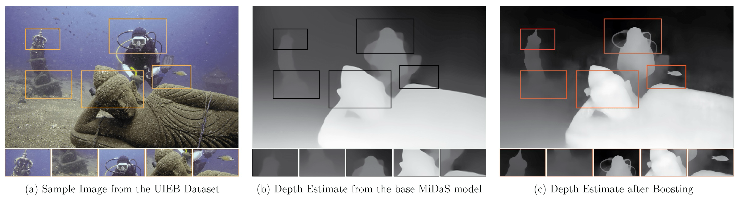
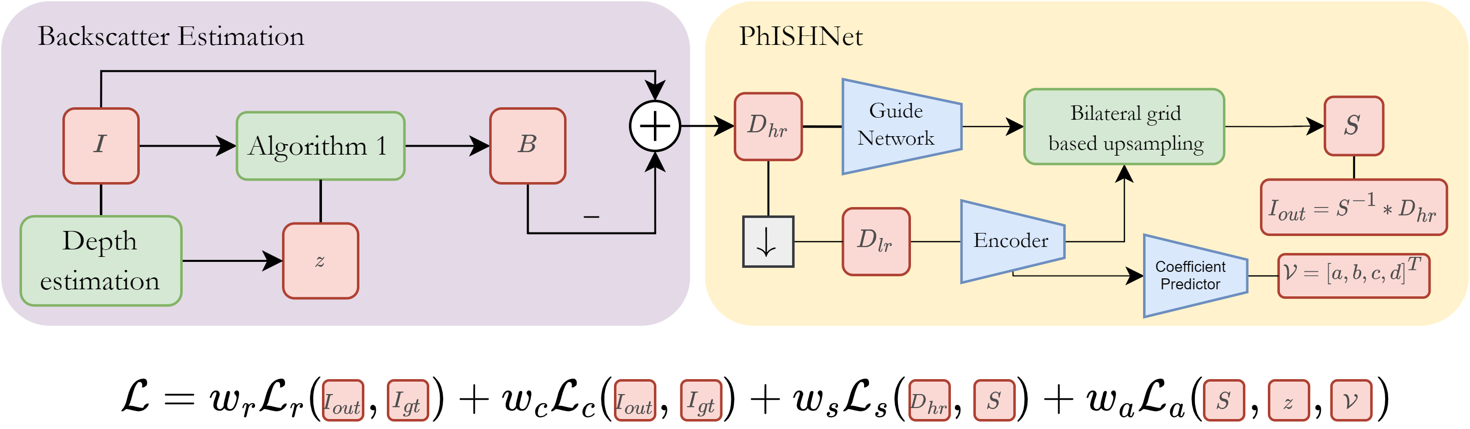
We first estimate and remove the backscatter component \(B\). The depth map \(z\) is obtained from an off-the-shelf monocular depth estimator (boosted MiDaS). The depth map is partitioned into 10 evenly spaced clusters; within each cluster, the darkest 1% of RGB triplets (where \(I \approx B\)) are collected into set \(\Omega\). An overestimate of backscatter is \(\hat{B}(\Omega) \approx I(\Omega)\), which follows:

\[ \hat{B} = \underbrace{J' \cdot e^{-\beta_{d'} z}}_{\text{Residual}} + B^\infty(1 - e^{-\beta_b z}) \tag{3} \]

The coefficients \(B^\infty, \beta_b, \beta_{d'}, J'\) are estimated by non-linear least squares fitting. The direct signal is then \(D_c = I_c - \hat{B}_c\).

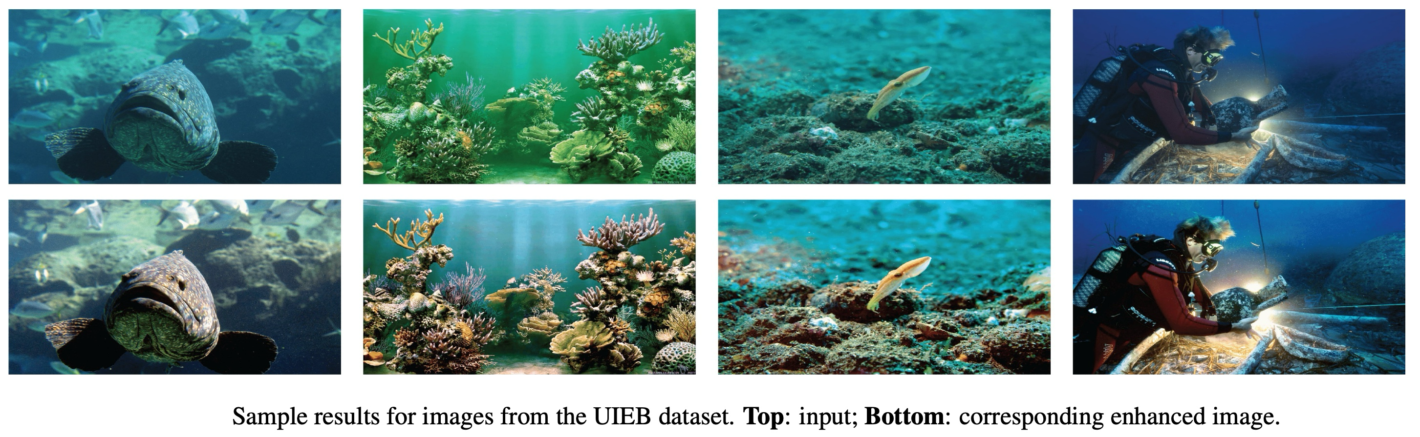
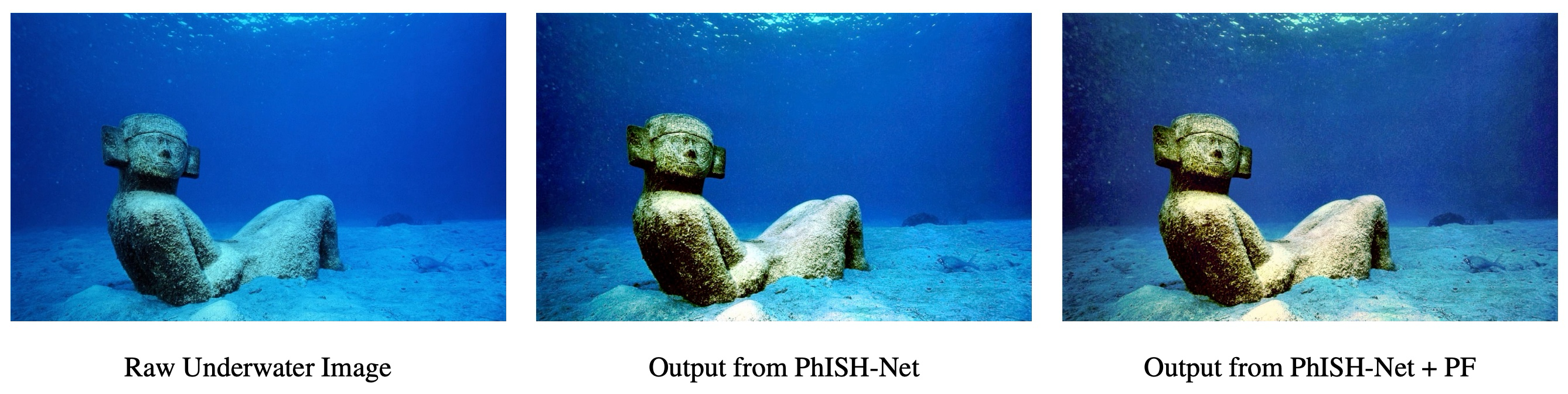
Impact of depth boosting on depth estimation — **Fig. 2: Impact of Depth Boosting.** (a) Sample image from the UIEB dataset. (b) Depth estimate from the base MiDaS model. (c) Depth estimate after boosting, showing finer detail for backscatter estimation.

PhISH-Net: Retinex-Based Enhancement

The direct signal \(D\) resembles a low-light underexposed image. Following the retinex model, we decompose \(D = S \ast \tilde{I}\) where \(S\) is the illumination map and \(\tilde{I}\) is the reflectance (enhanced image). PhISH-Net predicts a 3-channel illumination map \(S_{hr}\) from which the enhanced image is obtained as \(I_{out} = D_{hr} / (S_{hr} + \epsilon)\).

The network uses a lightweight convolutional encoder to extract features at low resolution. Local and global features are then used to predict bilateral grid coefficients, which are applied to a full-resolution guide map to produce \(S_{hr}\). This keeps most computation at low resolution while generating high-resolution outputs.

Wideband Attenuation Prior

To couple the deep enhancement with the physics of the UIFM, we introduce a novel loss that constrains the predicted illumination map to respect the known behavior of the attenuation coefficient \(\beta_d\). A coarse estimate of \(\beta_d\) can be derived from the predicted \(S_{hr}\) and depth \(z\):

\[ \hat{\beta}_d(z) = \frac{-\log S_{hr}}{z} \tag{4} \]

Sea-Thru established that \(\beta_d\) follows a two-term exponential decay with depth:

\[ \beta_d(z) = a \cdot e^{-b \cdot z} + c \cdot e^{-d \cdot z} \tag{5} \]

The wideband attenuation prior loss enforces this relationship:

\[ \mathcal{L}_a = \left\|\frac{-\log S_{hr}}{z} - (a e^{-bz} + c e^{-dz})\right\|^2 \tag{6} \]

The coefficients \(V = [a, b, c, d]\) are predicted by a learnable network from encoder features. The total training loss combines reconstruction, color, smoothness, and attenuation prior:

\[ \mathcal{L} = w_r \mathcal{L}_r + w_c \mathcal{L}_c + w_s \mathcal{L}_s + w_a \mathcal{L}_a \tag{7} \]

with \(w_r = 10,\ w_s = 2,\ w_c = 1,\ w_a = 0.5\).

PhISH-Net pipeline overview — **Fig. 3:** PhISH-Net pipeline. (1) Backscatter is estimated and removed using depth. (2) PhISH-Net predicts bilateral grid coefficients from the low-resolution direct signal, yielding a high-resolution illumination map and enhanced image via the retinex model.

Results

Comparison with State-of-the-Art

Method	PSNR↑	PSNR-L↑	SSIM↑	PCQI↑	UCIQE↑	UIQM↑	UICM↑	UIConM↑	CCF↑
UIEB Dataset
FUnIE-GAN	17.38	20.06	0.729	0.639	0.546	1.399	5.778	1.161	21.06
UW-GAN	16.23	19.15	0.764	0.719	0.566	1.347	5.555	1.122	22.84
UWCNN	12.02	13.78	0.647	0.392	0.506	1.065	1.922	0.940	11.00
HLRP	13.03	13.79	0.287	0.233	0.636	1.648	9.509	1.192	36.93
MLLE	18.11	19.47	0.799	0.911	0.604	1.629	4.827	1.012	36.27
IBLA	15.56	17.78	0.739	0.695	0.602	1.440	7.331	1.014	28.98
TOPAL	20.59	22.67	0.867	0.715	0.584	1.221	5.009	1.032	21.22
UDCP	11.93	12.73	0.644	0.612	0.596	1.573	7.199	1.175	27.14
Water-Net	18.70	19.72	0.862	0.693	0.571	1.264	5.064	1.063	16.50
ICSP	11.79	13.10	0.634	0.732	0.564	1.476	6.301	1.048	26.69
PhISH-Net	21.14	23.43	0.869	0.929	0.641	1.597	8.817	1.151	37.24
EUVP Dataset
FUnIE-GAN	20.56	27.47	0.887	0.893	0.509	1.555	4.098	1.250	29.23
UW-GAN	15.76	22.84	0.916	0.965	0.526	1.474	3.391	1.216	29.31
UWCNN	15.52	18.45	0.844	0.645	0.543	1.421	1.638	1.261	19.57
MLLE	14.25	16.19	0.613	1.030	0.588	1.730	2.991	0.776	36.22
IBLA	16.92	23.09	0.864	0.989	0.590	1.562	4.618	1.110	39.54
TOPAL	18.30	24.48	0.934	0.994	0.583	1.491	3.252	1.199	34.90
Water-Net	18.26	24.35	0.936	0.883	0.579	1.498	3.147	1.231	25.62
ICSP	12.13	14.51	0.671	0.980	0.575	1.590	4.092	0.973	41.29
PhISH-Net	20.92	27.47	0.856	1.038	0.592	1.593	4.357	1.151	38.86

Table 1: Image quality metrics on UIEB and EUVP datasets (all higher is better). PhISH-Net achieves the best PSNR, PSNR-L, and SSIM on UIEB, and is competitive across all metrics on EUVP.

Ablation Study

\(\mathcal{L}_r\)	\(\mathcal{L}_c\)	\(\mathcal{L}_s\)	\(\mathcal{L}_a\)	PSNR↑	SSIM↑
✓				20.80	0.830
✓	✓			20.86	0.832
✓	✓	✓		20.87	0.832
✓	✓	✓	✓	21.14	0.869

Table 2: Ablation of loss components on UIEB. The wideband attenuation prior \(\mathcal{L}_a\) provides the largest single gain, confirming the value of physics-based supervision.

Impact of Photofinishing

BibTeX

@InProceedings{chandrasekar2024phishnet,
  author    = {Chandrasekar, Aditya and Sreenivas, Manogna and Biswas, Soma},
  title     = {PhISH-Net: Physics Inspired System for High Resolution Underwater Image Enhancement},
  booktitle = {Winter Conference on Applications of Computer Vision},
  year      = {2024}
}